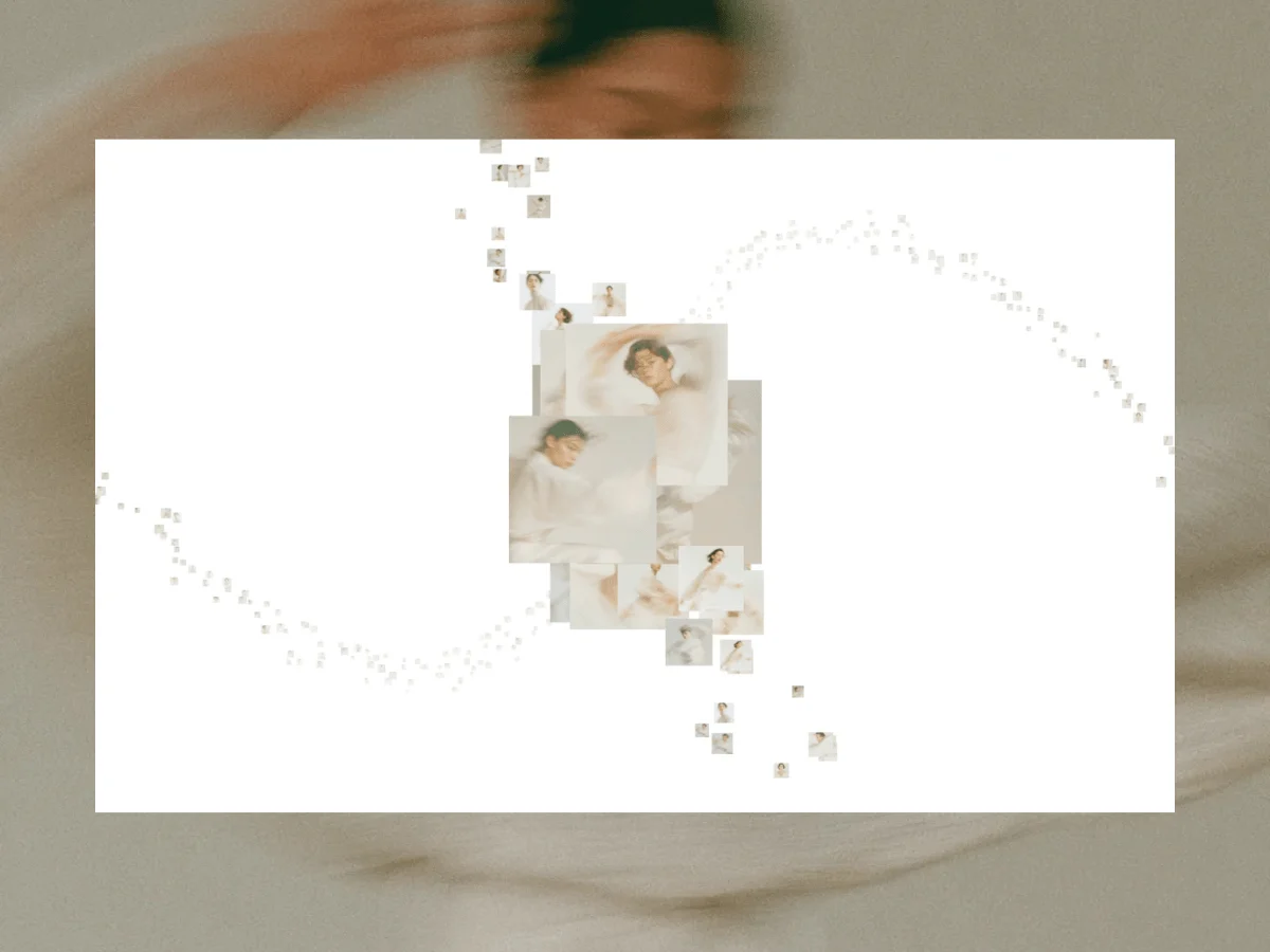
This tutorial delves into the creation of an interactive 3D gallery, distinguished by its dynamic camera movement that fluidly follows a custom-designed path. Images are strategically positioned along a curve meticulously crafted in Blender. The user’s scrolling action directly influences the camera’s traversal through this three-dimensional space. As elements approach the camera’s focal point, they magnify, simulating a natural focus effect, while other objects recede into the background, maintaining a sense of depth and perspective. The overall experience emulates a continuous camera dolly shot, where each scroll action propels the viewer further along the pre-defined path, fostering an immersive journey through a virtual environment. The technological backbone of this project relies on a synergistic combination of Blender for path creation, Three.js for rendering and scene management, and GSAP for sophisticated animation and scroll-driven interactions. The inspiration for this innovative approach is drawn from the captivating digital artwork produced by the creative studio BAXSTUDIO.
The Genesis of the 3D Gallery: From Blender to the Web
The foundation of this immersive experience is laid within the robust 3D modeling software, Blender. This initial phase involves the conceptualization and creation of the camera’s trajectory, a crucial element that dictates the rhythm and flow of the entire gallery.
Crafting the Camera Path in Blender
The process begins by introducing a Bezier curve within Blender. This fundamental shape serves as the blueprint for the camera’s movement. Users are encouraged to enter ‘Edit Mode’ to sculpt this curve into any desired form, be it a graceful spiral, a sinuous wave, a sharp, dramatic turn, or an extended straight segment. The inherent flexibility of the curve allows for a wide spectrum of user experiences, with each design choice directly influencing the pacing and visual narrative of the gallery. This creative decision-making process in Blender is paramount to defining the unique character of the final project.
Exporting the Path Data
Once the camera path is finalized in Blender, the next critical step is to translate this 3D data into a format that can be readily interpreted by web technologies. This is achieved by exporting the curve as a JSON file. To facilitate this export, users navigate to Blender’s ‘Scripting’ workspace and create a new Python script. The provided script leverages Blender’s API to extract the vertex coordinates of the active curve object.
import bpy
import json

obj = bpy.context.active_object
depsgraph = bpy.context.evaluated_depsgraph_get()
obj_eval = obj.evaluated_get(depsgraph)

# Ensure the object is a curve before proceeding
if obj.type == 'CURVE':
    # Evaluate the curve to get its mesh representation for vertex extraction
    mesh = obj_eval.to_mesh()

    points = []
    for v in mesh.vertices:
        # Apply the object's world matrix to vertex coordinates
        co = obj.matrix_world @ v.co
        # Remap Blender's coordinate system (Z-up) to Three.js (Y-up)
        points.append([round(co.x, 3), round(co.z, 3), round(-co.y, 3)])

    # Clean up the evaluated mesh
    obj_eval.to_mesh_clear()

    # Define the export path (ensure this directory exists)
    # For demonstration, we'll assume a relative path or a placeholder
    # In a real project, you would configure this path appropriately.
    # Example: path = "/path/to/your/project/public/paths/path1.json"
    path = "path1.json" # Placeholder for demonstration

    with open(path, "w") as f:
        json.dump(points, f)

    print(f"Exported len(points) points to path")
else:
    print("Selected object is not a curve. Please select a curve object.")
A pivotal line within this script is points.append([round(co.x, 3), round(co.z, 3), round(-co.y, 3)]). This operation addresses a fundamental difference in coordinate system conventions between Blender and Three.js. Blender utilizes a Z-up system, where the Z-axis represents verticality. Conversely, Three.js employs a Y-up system. Failing to account for this discrepancy would result in the entire exported curve being rotated incorrectly within the 3D scene, leading to erroneous camera movement. This remapping ensures that the spatial orientation of the path is preserved during the transition to the web environment.
Upon execution of this script with the curve object selected, a JSON file is generated. This file contains an array of precisely sampled points that define the camera’s journey. For instance, a snippet might look like [[-27.559, 0.0, -0.0], [-27.56, 0.02, -0.022], [-27.56, 0.04, -0.044], ...]. This JSON data is then placed within the public/paths/ directory of the web project, ready to be loaded and reconstructed in the subsequent stage.
Reconstructing the Path and Establishing the Scene with Three.js
With the camera path data in hand, the focus shifts to the web browser, where Three.js takes center stage to reconstruct the curve and build the interactive 3D environment.
Initializing the Rendering Environment
The first step involves setting up the core components of the Three.js scene: the renderer, the scene itself, and the camera.
const renderer = new THREE.WebGLRenderer( antialias: true );
renderer.setPixelRatio(Math.min(window.devicePixelRatio, 2));
renderer.setSize(window.innerWidth, window.innerHeight);
document.getElementById('canvas-container').appendChild(renderer.domElement); // Assuming a div with id 'canvas-container' exists

const scene = new THREE.Scene();
scene.background = new THREE.Color(0xffffff); // White background
scene.fog = new THREE.Fog(0xffffff, 10, 40); // Fading fog for depth perception

const camera = new THREE.PerspectiveCamera(60, window.innerWidth / window.innerHeight, 0.1, 200);
The renderer is configured for antialiasing to ensure smooth edges and its pixel ratio is adjusted for high-resolution displays. The scene is initialized with a white background and a fog effect. This fog, while not strictly essential for the core functionality, significantly enhances the sense of depth by gradually obscuring distant objects, contributing to a more immersive visual experience. The perspective camera is set up with a 60-degree field of view, defining the viewer’s visual range.
Defining Scene Parameters and Constants
A set of crucial constants is defined to govern the behavior and appearance of the gallery. These parameters allow for fine-tuning the experience and maintaining consistency across different configurations.
const SCALE = 16; // Scaling factor for Blender units to scene units
const TEX_VARIANTS = 12; // Number of unique image textures available
const textureLoader = new THREE.TextureLoader();
const textures = loadTextureVariants(TEX_VARIANTS, textureLoader); // Pre-load all textures

const TOTAL = 500; // Total number of image planes to be rendered
const CAM_Z = 10; // Offset for the camera along the Z-axis for optimal viewing
const FOCUS_DIST = 5.5; // Distance from the camera where planes begin to scale up
const MAX_SCALE = 14; // Maximum scale factor for planes within the focus zone
const Z_GATE = 11; // Depth threshold to filter out distant planes for performance

const LATERAL_OFFSET_RANGE = [-1, 1]; // Range for horizontal distribution of planes
const DEPTH_OFFSET_RANGE = [-0.75, 0.75]; // Range for depth distribution of planes
const SIZE_RANGE = [0.18, 0.4]; // Range for the size of individual planes
These constants control aspects such as the scaling of the Blender-imported path, the number of available image textures, the total number of planes to be displayed, camera positioning, and the parameters defining the focus effect and distribution of elements within the scene.
Loading and Reconstructing the Curve
The exported JSON data representing the camera path is asynchronously fetched. Upon successful retrieval, the buildCurve function reconstructs the smooth 3D curve using THREE.CatmullRomCurve3.
function toScaledVector3([x, y, z], scale)
  return new THREE.Vector3(x * scale, y * scale, z * scale);


function buildCurve(raw)
  const points = raw.map(p => toScaledVector3(p, SCALE));
  // The parameters for CatmullRomCurve3 are: points, closed, curveType, tension
  // 'true' indicates a closed curve (start and end points connect)
  // 'catmullrom' specifies the interpolation algorithm
  // '0.5' is the tension parameter, affecting how tightly the curve bends
  return new THREE.CatmullRomCurve3(points, true, 'catmullrom', 0.5);


async function init()
  const raw = await fetch('/paths/path1.json').then(r => r.json());
  const curve = buildCurve(raw);
  // ... rest of the initialization code
THREE.CatmullRomCurve3 is instrumental in generating a fluid and continuous path through a series of defined points. The constructor’s parameters, including whether the curve is closed, the type of interpolation, and the tension, all contribute to the final shape and smoothness of the camera’s movement.
Navigating the Curve: Position and Tangent
To accurately place and orient objects along the reconstructed curve, it’s essential to understand both the position and the direction of the curve at any given point. The getCurveFrame utility function provides this crucial information.
function getCurveFrame(curve, t)
  const pos = curve.getPoint(t); // Get the position along the curve at parameter t
  const tangent = curve.getTangent(t); // Get the tangent (direction) at parameter t

  // Calculate a normal vector perpendicular to the tangent in the XY plane.
  // This is achieved by rotating the tangent vector 90 degrees.
  // nx and ny represent the components of this local normal.
  const nx = -tangent.y;
  const ny = tangent.x;

  return  pos, nx, ny ;
This function takes the curve object and a normalized parameter t (ranging from 0 to 1) representing the progress along the curve. It returns the THREE.Vector3 position and the tangent vector at that point. Crucially, it also calculates a local normal vector (nx, ny) by rotating the tangent 90 degrees in the XY plane. This normal vector is vital for distributing planes laterally, ensuring they remain perpendicular to the path, even as the curve bends and twists.
Populating the Scene: Distributing Image Planes
With the curve established, the next phase involves populating the 3D environment with the visual content – the image planes. This process ensures an even distribution and dynamic appearance of the gallery elements.
Pre-loading Textures for Efficiency
To optimize performance and reduce loading times, all available image textures are loaded upfront when the application initializes.
function loadTextureVariants(count, loader)
  // Assuming images are named picture1.webp, picture2.webp, etc.
  return Array.from( length: count , (_, i) => loader.load(`/img/picture$i + 1.webp`));


// ... within init() function
const textureLoader = new THREE.TextureLoader();
const textures = loadTextureVariants(TEX_VARIANTS, textureLoader);
By loading all textures into memory at the start, the system avoids repeated network requests and GPU memory allocations for each individual plane. Each plane then simply selects a texture from this pre-loaded pool at random, ensuring efficient reuse of texture assets and minimizing overhead.
Creating and Positioning Image Planes
A total of TOTAL planes are generated and strategically placed along the reconstructed curve.
const planes = [];

for (let i = 0; i < TOTAL; i++)
  const t = i / TOTAL; // Parameter t for even distribution along the curve

  const  pos, nx, ny  = getCurveFrame(curve, t); // Get position and local normal

  // Apply random offsets for a more organic distribution
  const lateralOffset = randomBetween(...LATERAL_OFFSET_RANGE);
  const depthOffset = randomBetween(...DEPTH_OFFSET_RANGE);
  const size = randomBetween(...SIZE_RANGE);

  const mesh = new THREE.Mesh(
    new THREE.PlaneGeometry(size, size), // Plane geometry with random size
    new THREE.MeshBasicMaterial(
      map: textures[Math.floor(Math.random() * TEX_VARIANTS)], // Assign a random texture
      side: THREE.DoubleSide, // Render both sides of the plane
    )
  );

  // Position the plane using the curve's position and the calculated normal for lateral offset
  mesh.position.set(
    pos.x + nx * lateralOffset, // Lateral offset along the normal
    pos.y + ny * lateralOffset, // Lateral offset along the normal
    pos.z + depthOffset       // Offset along the curve's depth axis
  );

  // Store relevant data in userData for animation and reference
  mesh.userData.t = t;
  mesh.userData.lateralOffset = lateralOffset;
  mesh.userData.depthOffset = depthOffset;
  mesh.userData.setScale = createScaleAnimator(mesh); // Attach a GSAP animator for smooth scaling

  planes.push(mesh);
  scene.add(mesh);


// Helper function for random number generation within a range
function randomBetween(min, max)
  return Math.random() * (max - min) + min;
The planes are not rigidly positioned but are given slight random variations in lateral offset, depth, and size. This distribution is intelligently applied using the curve’s local normal vector, ensuring that the planes fan out perpendicular to the path, adapting to the curve’s geometry. This approach prevents unnatural clustering or spacing and contributes to a more visually appealing and organic arrangement. Furthermore, each plane’s userData property is populated with essential information, including its parameter t along the curve, its random offsets, and a pre-configured GSAP animator for smooth scaling transitions.
Implementing Dynamic Scaling with GSAP
To achieve the effect of images coming into focus, each plane is equipped with an individual scale animator created using gsap.quickTo().
function createScaleAnimator(mesh)
  const proxy =  value: 1 ; // A proxy object to animate
  return gsap.quickTo(proxy, 'value',
    duration: 0.4, // Smooth animation duration
    ease: 'power3.out', // Easing function for the animation
    onUpdate: () => mesh.scale.setScalar(proxy.value), // Update mesh scale on animation update
  );
gsap.quickTo() generates a highly optimized function that efficiently animates a specific property of an object towards a target value. Instead of creating a new animation tween for every scale adjustment, it reuses and updates an existing one. This is crucial for performance, as it prevents the creation of numerous short-lived tweens, especially when scale targets are frequently recalculated, as is the case in this dynamic gallery. The onUpdate callback ensures that the mesh’s scale is updated in real-time as the animation progresses, providing a fluid visual transition.
Scroll-Driven Camera Control: The Heart of Interactivity
The interactive element of the gallery is primarily driven by the user’s scroll input, which dictates the camera’s movement along the pre-defined path.
The Principle of Scroll-Based Navigation
The camera’s position is controlled by a single parameter, t, which interpolates from 0 to 1, representing the entire length of the curve. To ensure smooth and responsive navigation, two distinct values are maintained: camProxy.t, which represents the current smoothed camera position, and targetT, which reflects the raw, unfiltered scroll input. This separation allows for immediate reaction to user input while ensuring that the camera’s movement is visually fluid and not jerky.
const camProxy =  t: 0 ; // Proxy object for the camera's current position parameter
// gsap.quickTo creates a function that animates camProxy.t towards a target value.
const setCamT = gsap.quickTo(camProxy, 't',  duration: 1, ease: 'power3.out' );

let targetT = 0; // Stores the raw scroll input
const SENSITIVITY = 1 / (window.innerHeight * 4); // Sensitivity factor for scroll input
The SENSITIVITY constant plays a vital role in calibrating the scroll experience. By scaling it with window.innerHeight, the interaction remains consistent across devices of varying screen sizes, ensuring that scrolling the full viewport height results in a comparable advancement along the camera path.
Capturing Scroll Events with GSAP Observer
GSAP’s Observer plugin provides a unified and efficient mechanism for capturing user input across different devices and interaction types.
Observer.create(
  target: window, // Observe scroll events on the window
  type: 'wheel,touch,pointer', // Listen for wheel, touch, and pointer events
  onChange: (self) =>
    targetT += self.deltaY * SENSITIVITY; // Update targetT based on scroll delta
    setCamT(targetT); // Animate camProxy.t towards the new targetT
  ,
);
The Observer plugin abstracts away the complexities of handling various input events, providing a consistent deltaY value for scroll-like actions. On each input event, targetT is updated, and setCamT() is called. This function, powered by gsap.quickTo(), smoothly interpolates camProxy.t towards the targetT value over one second with a power3.out easing. This smooth transition is what gives the camera its characteristic gliding motion along the curve.
Updating the Camera in the Animation Loop
The animate function, called repeatedly via requestAnimationFrame, is responsible for updating the camera’s position based on the smoothed camProxy.t value.
function animate()
  requestAnimationFrame(animate);

  // Normalize t to ensure it stays within the [0, 1] range and handles wrapping.
  // The expression ((1 - camProxy.t) % 1 + 1) % 1 correctly maps the smoothed value
  // to the [0, 1] range, handling potential negative values or values exceeding 1.
  const t = ((1 - camProxy.t) % 1 + 1) % 1;

  const pathPos = curve.getPoint(t); // Get the 3D position on the curve
  // Set the camera's position, adding a Z offset for better viewing angle.
  camera.position.set(pathPos.x, pathPos.y, pathPos.z + CAM_Z);

  // ... (Code for updating plane scales)

  renderer.render(scene, camera); // Render the scene
The normalization of t is a critical aspect of handling closed curves. The expression ((1 - camProxy.t) % 1 + 1) % 1 ensures that t always remains within the valid range of 0 to 1, correctly handling cases where the camera wraps around the end of the curve back to the beginning. The CAM_Z offset positions the camera slightly in front of the curve, providing a more advantageous viewing perspective and preventing clipping through the planes.
Enhancing Depth: Scaling Images into Focus
The final layer of immersion is achieved through the dynamic scaling of image planes, making them appear to come into focus as they approach the camera.
The Focus Zone Mechanism
On each frame of the animation loop, every plane is evaluated to determine its proximity to the camera. If a plane falls within a predefined "focus zone," its scale is adjusted based on its distance. Planes outside this zone maintain their original size.
for (const plane of planes)
  const dx = camera.position.x - plane.position.x;
  const dy = camera.position.y - plane.position.y;
  const dz = Math.abs(camera.position.z - plane.position.z); // Absolute difference in Z depth
  const distXY = Math.sqrt(dx * dx + dy * dy); // Distance in the XY plane

  let dt = Math.abs(plane.userData.t - t); // Difference in curve parameter
  if (dt > 0.5)
    dt = 1 - dt; // Account for closed curve wrap-around


  // Determine if the plane is within the focus zone based on curve proximity, Z depth, and XY distance
  const isInFocusZone = dt < focusTGate && dz < Z_GATE && distXY < FOCUS_DIST;
  const targetScale = isInFocusZone
    ? computeFocusScale(distXY, FOCUS_DIST, MAX_SCALE) // Calculate scale if in focus
    : 1; // Default scale is 1 if outside focus zone

  plane.userData.setScale(targetScale); // Apply the calculated scale using the GSAP animator
A plane enters the focus zone only if it meets three criteria: its position along the curve (dt) is close enough to the camera’s current position, its depth difference (dz) is within a certain range, and its lateral distance (distXY) from the camera is within FOCUS_DIST. The dt calculation includes a crucial check to handle the wrap-around nature of a closed curve, ensuring that planes near the start and end are correctly identified as neighbors.
Calculating the Scale Factor
The computeFocusScale function calculates the target scale for planes within the focus zone, ensuring a smooth magnification effect.
function computeFocusScale(distance, maxDistance, maxScale)
  // Calculate a normalized proximity value (f=1 when distance=0, f=0 when distance=maxDistance)
  const f = 1 - distance / maxDistance;
  // Apply a cubic easing to f to concentrate the scaling effect near the camera
  // This results in a scale that ramps up quickly as the plane approaches the camera.
  // The scale ranges from 1 (original size) to maxScale.
  return 1 + Math.pow(f, 3) * (maxScale - 1);
This function generates a scale factor that increases non-linearly as the plane gets closer to the camera. By cubing the proximity value f, the scaling effect is concentrated towards the camera’s position. This means distant planes remain at their original size, while objects very close to the camera experience a rapid and pronounced enlargement, reinforcing the illusion of them coming into sharp focus.
Applying Scale Transitions with GSAP
The calculated targetScale is then applied to each plane using its pre-assigned GSAP animator.
plane.userData.setScale(targetScale);This ensures that the scale transitions are always smooth. Even though the targetScale is recalculated every frame, gsap.quickTo() interpolates the current scale towards this new target, creating a fluid visual effect rather than abrupt changes. This maintains the polished and professional feel of the interactive gallery.
Expanding the Experience: Advanced Features and Conclusion
The presented tutorial provides a robust foundation, but the demo includes additional functionalities that further enhance the user experience and demonstrate the extensibility of the core concepts.
Path Switching and Auto-Scroll Capabilities
The demo showcases the ability to switch between different pre-defined camera paths. When a new path is selected, the existing planes are smoothly redistributed along the new trajectory using GSAP’s animation capabilities. This transition is animated, ensuring a seamless visual flow rather than an abrupt jump. Furthermore, an auto-scroll feature is implemented, allowing the camera to move autonomously along the path. This is achieved by continuously incrementing targetT within the animation loop, leveraging the existing smoothing logic of gsap.quickTo() for a continuous and engaging dolly shot experience.
Conclusion: The Power of the Path
The creation of this interactive 3D gallery underscores the profound impact that a simple, well-designed path can have on an entire user experience. Each technology employed plays a distinct and vital role: Blender for the initial creative design of the path, Three.js for the reconstruction and rendering of the 3D environment, and GSAP for bringing the scene to life with dynamic animations and responsive scroll interactions. The true artistic control lies within the shape of the curve itself. By iterating on the path design in Blender and re-exporting, creators can fundamentally alter the rhythm, perspective, and narrative of the gallery, all while the underlying implementation remains consistent. The experience is ultimately defined by the path, making it a powerful tool for immersive storytelling in the digital realm.